Importance Weighted Autoencoders

reimplementation
VAE
IWAE
generative
Author

borea17

Published

January 10, 2021

Burda et al. (2016) introduce the Importance Weighted Autoencoder (IWAE) as a simple modification in the training of variational autoencoders (VAEs). Notably, they proved that this modification leads to a strictly tighter lower bound on the data log-likelihood. Furthermore, the standard VAE formulation is contained within the IWAE framework as a special case. In essence, the modification consists of using multiple samples from the recognition network / encoder and adapting the loss function with importance-weighted sample losses. In their experiments, they could emprically validate that employing IWAEs leads to improved test log-likelihoods and richer latent space representations compared to VAEs.

Model Description

An IWAE can be understood as a standard VAE in which multiple samples are drawn from the encoder distribution \(q_{\boldsymbol{\phi}} \Big( \textbf{z} | \textbf{x} \Big)\) and then fed through the decoder \(p_{\boldsymbol{\theta}} \Big( \textbf{z} | \textbf{x} \Big)\). In principle, this modification has been already proposed in the original VAE paper by Kingma and Welling (2013). However, Burda et al. (2016) additionally proposed to use a different objective function. The empirical objective function can be understood as the data log-likelihood \(\log p_{\boldsymbol{\theta}} (\textbf{x})\) where the sampling distribution is exchanged to \(q_{\boldsymbol{\phi}} \Big( \textbf{z} | \textbf{x} \Big)\) via the method of importance sampling.

High-Level Overview

The IWAE framework builds upon a standard VAE architecture. There are two neural networks as approximations for the encoder \(q_{\boldsymbol{\phi}} \left(\textbf{z} | \textbf{x} \right)\) and the decoder distribution \(p_{\boldsymbol{\theta}} \left( \textbf{x} | \textbf{z} \right)\). More precisely, the networks estimate the parameters that parametrize these distributions. Typically, the latent distribution is assumed to be a Gaussian \(q_{\boldsymbol{\phi}} \left(\textbf{z} | \textbf{x} \right) \sim \mathcal{N}\left( \boldsymbol{\mu}_{\text{E}}, \text{diag} \left( \boldsymbol{\sigma}^2_{\text{E}}\right) \right)\) such that the encoder network estimates its the mean \(\boldsymbol{\mu}\_{\text{E}}\) and variance1 \(\boldsymbol{\Sigma} = \text{diag} \left(\boldsymbol{\sigma}^2_{\text{E}}\right)\). To allow for backpropagation, we apply the reparametrization trick to the latent distribution which essentially consist of transforming samples from some (fixed) random distribution, e.g. \(\boldsymbol{\epsilon} \sim \mathcal{N} \left(\textbf{0}, \textbf{I} \right)\), into the desired distribution using a deterministic mapping.

The main difference between a VAE and an IWAE lies in the objective function which is explained in more detail in the next section.

VAE/IWAE Architecture

Derivation

Let \(\textbf{X} = \{\textbf{x}^{(i)}\}_{i=1}^N\) denote a dataset of \(N\) i.i.d. samples where each observed datapoint \(\textbf{x}^{(i)}\) is obtained by first sampling a latent vector \(\textbf{z}\) from the prior \(p_{\boldsymbol{\theta}}(\textbf{z})\) and then sampling \(\textbf{x}^{(i)}\) itself from the scene model \(p_{\boldsymbol{\theta}} \Big( \textbf{x} | \textbf{z} \Big)\). Now we introduce an auxiliary distribution \(q_{\boldsymbol{\phi}} \Big( \textbf{z} | \textbf{x} \Big)\) (with its own paramaters) as an approximation to the true, but unknown posterior \(p_{\boldsymbol{\theta}} \left( \textbf{z} | \textbf{x} \right)\). Accordingly, the data likelihood of a one sample \(\textbf{x}^{(i)}\) can be stated as follows

\[ p_{\boldsymbol{\theta}} (\textbf{x}^{(i)}) = \mathbb{E}_{\textbf{z} \sim p_{\boldsymbol{\theta}} \Big(\textbf{z} \Big)} \Big[ p_{\boldsymbol{\theta}} \left( \textbf{z} | \textbf{x}^{(i)} \right) \Big] = \int p_{\boldsymbol{\theta}} (\textbf{z}) p_{\boldsymbol{\theta}} \left( \textbf{z} | \textbf{x}^{(i)} \right) d\textbf{z} = \int p_{\boldsymbol{\theta}} \left(\textbf{x}^{(i)} , \textbf{z} \right) d\textbf{z} \]

Now, we use the simple trick of importance sampling to change the sampling distribution into the approximated posterior, i.e.,

\[ p_{\boldsymbol{\theta}} \left( \textbf{x}^{(i)}\right) = \int \frac {p_{\boldsymbol{\theta}} \left(\textbf{x}^{(i)} , \textbf{z} \right)} {q_{\boldsymbol{\phi}} \left( \textbf{z} | \textbf{x}^{(i)} \right)} q_{\boldsymbol{\phi}} \left( \textbf{z} | \textbf{x}^{(i)} \right) d\textbf{z} = \mathbb{E}_{\textbf{z} \sim q_{\boldsymbol{\phi}} \left( \textbf{z} | \textbf{x}^{(i)} \right)} \left[ \frac {p_{\boldsymbol{\theta}} \left(\textbf{x}^{(i)} , \textbf{z} \right)} {q_{\boldsymbol{\phi}} \left( \textbf{z} | \textbf{x}^{(i)} \right)} \right] \]

VAE Formulation

In the standard VAE approach, we use the evidence lower bound (ELBO) on \(\log p_{\boldsymbol{\theta}} \Big( \textbf{x}\Big)\) as the objective function. This can be derived by applying Jensen’s Inequality on the data log-likelihood:

\[ \log p_{\boldsymbol{\theta}} \left( \textbf{x}^{(i)} \right) = \log \mathbb{E}_{\textbf{z} \sim q_{\boldsymbol{\phi}} \left( \textbf{z} | \textbf{x}^{(i)} \right)} \left[ \frac {p_{\boldsymbol{\theta}} \left(\textbf{x}^{(i)} , \textbf{z} \right)} {q_{\boldsymbol{\phi}} \left( \textbf{z} | \textbf{x}^{(i)} \right)} \right] \ge \mathbb{E}_{\textbf{z} \sim q_{\boldsymbol{\phi}} \left( \textbf{z} | \textbf{x}^{(i)} \right)} \left[ \log \frac {p_{\boldsymbol{\theta}} \left(\textbf{x}^{(i)} , \textbf{z} \right)} {q_{\boldsymbol{\phi}} \left( \textbf{z} | \textbf{x}^{(i)} \right)} \right] = \mathcal{L}^{\text{ELBO}} \]

Using simple algebra, this can be rearranged into

\[ \mathcal{L}^{\text{ELBO}}\left(\boldsymbol{\theta}, \boldsymbol{\phi}; \textbf{x}^{(i)} \right) = \underbrace{ \mathbb{E}_{\textbf{z} \sim q_{\phi} \left( \textbf{z}| \textbf{x}^{(i)} \right)} \left[ \log p_{\boldsymbol{\theta}} \Big(\textbf{x}^{(i)} | \textbf{z} \Big) \right]}_{ \text{Reconstruction Accuracy}} - \underbrace{ D_{KL} \left( q_{\phi} \Big( \textbf{z} | \textbf{x}^{(i)} \Big) || p_{\boldsymbol{\theta}} \Big( \textbf{z} \Big) \right) }_{\text{Regularization}} \]

While the regularization term can usually be solved analytically, the reconstruction accuracy in its current formulation poses a problem for backpropagation: Gradients cannot backpropagate through a sampling operation. To circumvent this problem, the standard VAE formulation includes the reparametrization trick:
Substitute sampling \(\textbf{z} \sim q_{\boldsymbol{\phi}}\) by using a deterministic mapping \(\textbf{z} = g_{\boldsymbol{\phi}} (\boldsymbol{\epsilon}, \textbf{x})\) with the differential transformation \(g_{\boldsymbol{\phi}}\) of an auxiliary noise variable \(\boldsymbol{\epsilon}\) with \(\boldsymbol{\epsilon}\sim p(\boldsymbol{\epsilon})\).


As a result, we can rewrite the EBLO as follows

\[ \mathcal{L}^{\text{ELBO}}\left(\boldsymbol{\theta}, \boldsymbol{\phi}; \textbf{x}^{(i)} \right) = \mathbb{E}_{\boldsymbol{\epsilon} \sim p \left( \boldsymbol{\epsilon} \right)} \left[ \log p_{\boldsymbol{\theta}} \Big(\textbf{x}^{(i)} | g_{\boldsymbol{\phi}} \left( \boldsymbol{\epsilon}, \textbf{x}^{(i)} \right) \Big) \right] - D_{KL} \left( q_{\phi} \Big( \textbf{z} | \textbf{x}^{(i)} \Big) || p_{\boldsymbol{\theta}} \Big( \textbf{z} \Big) \right) \]

Lastly, the expectation is approximated using Monte-Carlo integration, leading to the standard VAE objective

\[ \begin{align} \widetilde{\mathcal{L}}^{\text{VAE}}_k \left(\boldsymbol{\theta}, \boldsymbol{\phi}; \textbf{x}^{(i)}\right) &= \frac {1}{k} \sum_{l=1}^{k} \log p_{\boldsymbol{\theta}}\left( \textbf{x}^{(i)}| g_{\boldsymbol{\phi}} \left( \boldsymbol{\epsilon}^{(l)}, \textbf{x}^{(i)} \right)\right) -D_{KL} \left( q_{\boldsymbol{\phi}} \left( \textbf{z} | \textbf{x}^{(i)} \right), p_{\boldsymbol{\theta}} (\textbf{z}) \right)\\ &\text{with} \quad \boldsymbol{\epsilon}^{(l)} \sim p(\boldsymbol{\epsilon}) \end{align} \]

Note that commonly \(k=1\) in VAEs as long as the minibatch size is large enough. As stated by Kingma and Welling (2013):

Quote

We found that the number of samples per datapoint can be set to 1 as long as the minibatch size was large enough.

IWAE Formulation

Before we introduce the IWAE estimator, remind that the Monte-Carlo estimator of the data likelihood (when the sampling distribution is changed via importance sampling, see Derivation) is given by

\[ p_{\boldsymbol{\theta}} (\textbf{x} ) = \mathbb{E}_{\textbf{z} \sim q_{\boldsymbol{\phi}} \left( \textbf{z} | \textbf{x}^{(i)} \right)} \left[ \frac {p_{\boldsymbol{\theta}} \left(\textbf{x} , \textbf{z} \right)} {q_{\boldsymbol{\phi}} \left( \textbf{z} | \textbf{x} \right)} \right] \approx \frac {1}{k} \sum_{l=1}^{k} \frac {p_{\boldsymbol{\theta}} \left(\textbf{x} , \textbf{z}^{(l)} \right)} {q_{\boldsymbol{\phi}} \left( \textbf{z}^{(l)} | \textbf{x} \right)} \quad \text{with} \quad \textbf{z}^{(l)} \sim q_{\boldsymbol{\phi}} \left( \textbf{z} | \textbf{x}^{(i)} \right) \]

As a result, the data log-likelihood estimator for one sample \(\textbf{x}^{(i)}\) can be stated as follows

\[ \begin{align} \log p_{\boldsymbol{\theta}} (\textbf{x}^{(i)} ) &\approx \log \left[ \frac {1}{k} \sum_{l=1}^{k} \frac {p_{\boldsymbol{\theta}} \left(\textbf{x}^{(i)} , \textbf{z}^{(i, l)} \right)} {q_{\boldsymbol{\phi}} \left( \textbf{z}^{(i, l)} | \textbf{x}^{(i)} \right)}\right] = \widetilde{\mathcal{L}}^{\text{IWAE}}_k \left( \boldsymbol{\theta}, \boldsymbol{\phi}; \textbf{x}^{(i)} \right) \\ &\text{with} \quad \textbf{z}^{(i, l)} \sim q_{\boldsymbol{\phi}} \left( \textbf{z} | \textbf{x}^{(i)} \right) \end{align} \]

which leads to an empirical estimate of the IWAE objective. However, Burda et al. (2016) do not use the data log-likelihood in its plain form as the true IWAE objective. Instead they introduce the IWAE objective as follows

\[ \mathcal{L}^{\text{IWAE}}_k \left(\boldsymbol{\theta}, \boldsymbol{\phi}; \textbf{x}^{(i)}\right) = \mathbb{E}_{\textbf{z}^{(1)}, \dots, \textbf{z}^{(k)} \sim q_{\phi} \left( \textbf{z}| \textbf{x}^{(i)} \right)} \left[ \log \frac {1}{k} \sum_{l=1}^k \frac {p_{\boldsymbol{\theta}} \left(\textbf{x}^{(i)}, \textbf{z}^{(l)}\right)} {q_{\phi} \left( \textbf{z}^{(l)} | \textbf{x}^{(i)} \right)} \right] \]

For notation purposes, they denote

\[ \text{(unnormalized) importance weights:} \quad {w}^{(i, l)} = \frac {p_{\boldsymbol{\theta}} \left(\textbf{x}^{(i)}, \textbf{z}^{(l)}\right)} {q_{\phi} \left( \textbf{z}^{(l)} | \textbf{x}^{(i)} \right)} \]

By applying Jensen’s Inequality, we can see that in fact the (true) IWAE estimator is merely a lower-bound on the plain data log-likelihood

\[ \mathcal{L}^{\text{IWAE}}_k \left( \boldsymbol{\theta}, \boldsymbol{\phi}; \textbf{x}^{(i)} \right) = \mathbb{E} \left[ \log \frac {1}{k} \sum_{l=1}^{k} {w}^{(i, l)}\right] \le \log \mathbb{E} \left[ \frac {1}{k} \sum_{l=1}^{k} {w}^{(i,l)} \right] = \log p_{\boldsymbol{\theta}} \left( \textbf{x}^{(i)} \right) \]

They could prove that with increasing \(k\) the lower bound gets strictly tighter and approaches the true data log-likelihood in the limit of \(k \rightarrow \infty\). Note that since the empirical IWAE estimator \(\widetilde{\mathcal{L}}_k^{\text{IWAE}}\) can be understood as a Monte-Carlo estimator on the true data log-likelihood, in the empirical case this property can simply be deduced from the properties of Monte-Carlo integration.

What is motivation of the true IWAE objective?

A very well explanation is given by Domke and Sheldon (2018). Starting from the property

\[ p(\textbf{x}) = \mathbb{E} \Big[ w \Big] = \mathbb{E}_{\textbf{z} \sim q_{\boldsymbol{\phi}} \left( \textbf{z} | \textbf{x}^{(i)} \right)} \left[ \frac {p_{\boldsymbol{\theta}} \left(\textbf{x} , \textbf{z} \right)} {q_{\boldsymbol{\phi}} \left( \textbf{z} | \textbf{x} \right)} \right] \]

We derived the ELBO using Jensen’s inequality

\[ \log p(\textbf{x}) \ge \mathbb{E} \Big[ \log w \Big] = \text{ELBO} \Big[ q || p \Big] \]

Suppose that we could make \(w\) more concentrated about its mean \(p(\textbf{x})\). Clearly, this would yield a tighter lower bound when applying Jensen’s Inequality.

(rhetorical break)

Can we make \(w\) more concentrated about its mean? YES, WE CAN.

For example using the sample average \(w_k = \frac {1}{k} \sum_{i=1}^k w^{(i)}\). This leads directly to the true IWAE objective

\[ \log p(\textbf{x}) \ge \mathbb{E} \Big[ \log w_k \Big] = \mathbb{E} \left[ \log \frac {1}{k} \sum_{i=1}^{k} w^{(i)} \right] = \mathcal{L}^{\text{IWAE}}_k \]

IWAE objective and plain log-likelihood lead to the same empirical estimate. How?

Here it gets interesting. A closer analysis on the IWAE bound by Nowozin (2018) revealed the following property

\[ \begin{align} &\quad \mathcal{L}_k^{\text{IWAE}} = \log p(\textbf{x}) - \frac {1}{k} \frac {\mu_2}{2\mu^2} + \frac {1}{k^2} \left( \frac {\mu_3}{3\mu^3} - \frac {3\mu_2^2}{4\mu^4} \right) + \mathcal{O}(k^{-3})\\ &\text{with} \quad \mu = \mathbb{E}_{\textbf{z} \sim q_{\boldsymbol{\phi}}} \left[ \frac {p_{\boldsymbol{\theta}}\left( \textbf{x}, \textbf{z} \right)}{q_{\boldsymbol{\phi}} \left( \textbf{z} | \textbf{x} \right)} \right] \quad \mu_i = \mathbb{E}_{\textbf{z} \sim q_{\boldsymbol{\phi}}} \left[ \left( \frac {p_{\boldsymbol{\theta}}\left( \textbf{x}, \textbf{z} \right)}{q_{\boldsymbol{\phi}} \left( \textbf{z} | \textbf{x} \right)} - \mathbb{E}_{\textbf{z} \sim q_{\boldsymbol{\phi}}} \left[ \frac {p_{\boldsymbol{\theta}}\left( \textbf{x}, \textbf{z} \right)}{q_{\boldsymbol{\phi}} \left( \textbf{z} | \textbf{x} \right)} \right] \right)^2 \right] \end{align} \]

Thus, the true objective is a biased - in the order of \(\mathcal{O}\left(k^{-1}\right)\) - and consistent estimator of the marginal log likelihood \(\log p(\textbf{x})\). The empirical estimator of the true IWAE objective is basically a special Monte-Carlo estimator (only one sample per \(k\)) on the true IWAE objective. It is more or less luck that we can formulate the same empirical objective and interpret it differently as the Monte-Carlo estimator (with \(k\) samples) on the data log-likelihood.

Let us take a closer look on how to compute gradients (fast) for the empirical estimate of the IWAE objective:

\[ \begin{align} \nabla_{\boldsymbol{\phi}, \boldsymbol{\theta}} \widetilde{\mathcal{L}}_k^{\text{IWAE}} \left( \boldsymbol{\theta}, \boldsymbol{\phi}; \textbf{x}^{(i)} \right) &= \nabla_{\boldsymbol{\phi}, \boldsymbol{\theta}} \log \frac {1}{k} \sum_{l=1}^k w^{(i,l)} \left( \textbf{x}^{(i)}, \textbf{z}^{(i, l)}_{\boldsymbol{\phi}}, \boldsymbol{\theta} \right) \quad \text{with} \quad \textbf{z}^{(i, l)} \sim q_{\boldsymbol{\phi}} \left(\textbf{z} | \textbf{x}^{(i)} \right)\\ &\stackrel{\text{(*)}}{=} \sum_{l=1}^{k} \frac {w^{(i, l)}}{\sum_{m=1}^{k} w^{(i, m)}} \nabla_{\boldsymbol{\phi}, \boldsymbol{\theta}} \log w^{(i,l)} = \sum_{l=1}^{k} \widetilde{w}^{(i, l)} \nabla_{\boldsymbol{\phi}, \boldsymbol{\theta}} \log w^{(i,l)}, \end{align} \]

where we introduced the following notation

\[ \text{(normalized) importance weights:} \quad \widetilde{w}^{(i, l)} = \frac {w^{(i,l)}}{\sum_{m=1}^k w^{(i, m)}} \]

\((*)\): Gradient Derivation:

\[ \begin{align} \frac {\partial \left[ \log \frac {1}{k} \sum_i^{k} w_i \left( \boldsymbol{\theta} \right) \right]}{\partial \boldsymbol{\theta}} &\stackrel{\text{chain rule}}{=} \frac {\partial \log a}{\partial a} \sum_{i}^{k} \frac {\partial a}{\partial w_i} \frac {\partial w_i}{\partial \boldsymbol{\theta}} \quad \text{with} \quad a = \frac {1}{k} \sum_{i}^k w_i (\boldsymbol{\theta})\\ &= \frac {k}{\sum_l^k w_l} \sum_{i}^{k}\frac {1}{k} \frac {\partial w_i (\boldsymbol{\theta})}{\partial \boldsymbol{\theta}} = \frac {1}{\sum_l^k w_l} \sum_{i}^{k} \frac {\partial w_i (\boldsymbol{\theta})}{\partial \boldsymbol{\theta}} \end{align} \]

Lastly, we use the following identity

\[ \frac {\partial w_i (\boldsymbol{\theta})}{\partial \boldsymbol{\theta}} = w_i (\boldsymbol{\theta}) \cdot \frac {\partial \log w_i (\boldsymbol{\theta})}{\partial \boldsymbol{\theta}} \stackrel{\text{chain rule}}{=} w_i (\boldsymbol{\theta}) \cdot \frac {1}{w_i (\boldsymbol{\theta})} \cdot \frac {\partial w_i (\boldsymbol{\theta})}{\partial \boldsymbol{\theta}} = \frac {\partial w_i (\boldsymbol{\theta})}{\partial \boldsymbol{\theta}} \]

Similar to VAEs, this formulation poses a problem for backpropagation due to the sampling operation. We use the same reparametrization trick to circumvent this problem and obtain a low variance update rule:

\[ \begin{align} \nabla_{\boldsymbol{\phi}, \boldsymbol{\theta}} \widetilde{\mathcal{L}}_k^{\text{IWAE}} &= \sum_{l=1}^{k} \widetilde{w}^{(i, l)} \nabla_{\boldsymbol{\phi}, \boldsymbol{\theta}} \log w^{(i,l)} \left( \textbf{x}^{(i)}, \textbf{z}_{\boldsymbol{\phi}}^{(i,l)}, \boldsymbol{\theta} \right) \quad \text{with} \quad \textbf{z}^{(i,l)} \sim q_{\boldsymbol{\phi}} \left(\textbf{z} | \textbf{x}^{(i)} \right)\\ &= \sum_{l=1}^k \widetilde{w}^{(i,l)} \nabla_{\boldsymbol{\phi}, \boldsymbol{\theta}} \log w^{(i,l)} \left(\textbf{x}^{(i)}, g_{\boldsymbol{\phi}} \left( \textbf{x}^{(i)}, \boldsymbol{\epsilon}^{(l)}\right), \textbf{x}^{(i)} \right), \quad \quad \boldsymbol{\epsilon} \sim p(\boldsymbol{\epsilon}) \end{align} \]

To make things clearer for the implementation, let us unpack the log

\[ \log w^{(i,l)} = \log \frac {p_{\boldsymbol{\theta}} \left(\textbf{x}^{(i)}, \textbf{z}^{(l)}\right)} {q_{\boldsymbol{\phi}} \left( \textbf{z}^{(l)} | \textbf{x}^{(i)} \right)} = \underbrace{\log p_{\boldsymbol{\theta}} \left (\textbf{x}^{(i)} | \textbf{z}^{(l)} \right)}_{\text{NLL}} + \log p_{\boldsymbol{\theta}} \left( \textbf{z}^{(l)} \right) - \log q_{\boldsymbol{\phi}} \left( \textbf{z}^{(l)} | \textbf{x}^{(i)} \right) \]

Before, we are going to implement this formulation, let us look whether we can separate out the KL divergence for the true IWAE objective of Burda et al. (2016). Therefore, we state the update for the true objective:

\[ \begin{align} \nabla_{\boldsymbol{\phi}, \boldsymbol{\theta}} \mathcal{L}_k^{\text{IWAE}} &= \nabla_{\boldsymbol{\phi}, \boldsymbol{\theta}} \mathbb{E}_{\textbf{z}^{(1)}, \dots, \textbf{z}^{(l)}} \left[ \log \frac {1}{k} \sum_{l=1}^{k} w^{(l)} \left( \textbf{x}, \textbf{z}^{(l)}_{\boldsymbol{\phi}}, \boldsymbol{\theta} \right) \right]\\ &= \mathbb{E}_{\textbf{z}^{(1)}, \dots, \textbf{z}^{(l)}} \left[ \sum_{l=1}^{k} \widetilde{w}_i \nabla_{\boldsymbol{\phi}, \boldsymbol{\theta}} \log w^{(l)} \left( \textbf{x}, \textbf{z}_{\boldsymbol{\phi}}^{(l)}, \boldsymbol{\theta} \right) \right]\\ &=\sum_{l=1}^{k} \widetilde{w}_i \mathbb{E}_{\textbf{z}^{(l)}} \left[ \nabla_{\boldsymbol{\phi}, \boldsymbol{\theta}} \log w^{(l)} \left( \textbf{x}, \textbf{z}_{\boldsymbol{\phi}}^{(l)}, \boldsymbol{\theta} \right) \right]\\ &\neq \sum_{l=1}^{k} \widetilde{w}_i \nabla_{\boldsymbol{\phi}, \boldsymbol{\theta}} \mathbb{E}_{\textbf{z}^{(l)}} \left[ \log w^{(l)} \left( \textbf{x}, \textbf{z}_{\boldsymbol{\phi}}^{(l)}, \boldsymbol{\theta} \right) \right] \end{align} \]

Unfortunately, we cannot simply move the gradient outside the expectation. If we could, we could simply rearrange the terms inside the expectation as in the standard VAE case.


Let us look, what would happen, if we were to describe the true IWAE estimator as the data log-likelihood \(\log p \left( \textbf{x} \right)\) in which the sampling distribution is exchanged via importance sampling:

\[ \begin{align} \nabla_{\boldsymbol{\phi}, \boldsymbol{\theta}} \log p \left( \textbf{x}^{(i)} \right) &= \nabla_{\boldsymbol{\phi}, \boldsymbol{\theta}} \log \mathbb{E}_{\textbf{z} \sim q_{\boldsymbol{\phi}} \left( \textbf{z} | \textbf{x}^{(i)}\right)} \left[ w (\textbf{x}^{(i)}, \textbf{z}, \boldsymbol{\theta})\right]\\ &\neq \nabla_{\boldsymbol{\phi}, \boldsymbol{\theta}} \mathbb{E}_{\textbf{z} \sim q_{\boldsymbol{\phi}} \left( \textbf{z} | \textbf{x}^{(i)}\right)} \left[ \log w (\textbf{x}^{(i)}, \textbf{z}, \boldsymbol{\theta})\right] \end{align} \]

Here, we also cannot separate the KL divergence out, since we cannot simply move the log inside the expectation.

Implementation

Let’s put this into practice and compare the standard VAE with an IWAE. We are going to perform a very similar experiment to the density estimation experiment by Burda et al. (2016), i.e., we are going to train both a VAE and IWAE with different number of samples \(k\in \{1, 10\}\) on the binarized MNIST dataset.

Dataset

Let’s first build a binarized version of the MNIST dataset. As noted by Burda et al. (2016), the generative modeling literature is inconsistent about the method of binarization. We employ the same procedure as Burda et al. (2016): binary-valued observations are sampled with expectations equal to the real values in the training set:

Code
import torch.distributions as dists
import torch
from torchvision import datasets, transforms


class Binarized_MNIST(datasets.MNIST):
    def __init__(self, root, train, transform=None, target_transform=None, download=False):
        super(Binarized_MNIST, self).__init__(root, train, transform, target_transform, download)

    def __getitem__(self, idx):
        img, target = super().__getitem__(idx)
        return dists.Bernoulli(img).sample().type(torch.float32)
Binarized MNIST Dataset

Model Implementation

  • VAE Implementation

    The VAE implementation is straightforward. For later evaluation, I added create_latent_traversal and compute_marginal_log_likelihood. The ladder computes the marginal log-likelihood \(\log p(\textbf{x})\) in which the sampling distribution is exchanged to the approximated posterior \(q_{\boldsymbol{\phi}} \left( \textbf{z} | \textbf{x}\right )\) using the standard Monte-Carlo estimator, i.e.,

    \[ \log p(\textbf{x}) = \mathbb{E}_{z\sim q_{\boldsymbol{\phi}}} \left[ \frac {p_{\boldsymbol{\theta}} \left(\textbf{x}, \textbf{z}\right)} {q_{\boldsymbol{\phi}} \left( \textbf{z} | \textbf{x} \right)} \right] \approx \log \left[ \frac {1}{k} \sum_{l=1}^k w^{(l)} \right] = \mathcal{L}^{\text{IWAE}}_k (\textbf{x}) \]

    Remind that this formulation equals the empirical IWAE estimator. However, we can only compute the (unnormalized) logarithmic importance weights

    \[ \log w^{(i,l)} = \log \frac {p_{\boldsymbol{\theta}} \left(\textbf{x}^{(i)}, \textbf{z}^{(l)}\right)} {q_{\boldsymbol{\phi}} \left( \textbf{z}^{(l)} | \textbf{x}^{(i)} \right)} = \log p_{\boldsymbol{\theta}} \left (\textbf{x}^{(i)} | \textbf{z}^{(l)} \right) + \log p_{\boldsymbol{\theta}} \left( \textbf{z}^{(l)} \right) - \log q_{\boldsymbol{\phi}} \left( \textbf{z}^{(l)} | \textbf{x}^{(i)} \right) \]

    Accordingly, we compute the marginal log-likelihood as follows

    \[ \begin{align} \widetilde{\mathcal{L}}^{\text{IWAE}}_k \left( \boldsymbol{\theta}, \boldsymbol{\phi}; \textbf{x}^{(i)} \right) &= \underbrace{\log 1}_{=0} - \log k + \log \left( \sum_{i=1}^k w^{(i,l)} \right) \\ &= -\log k + \underbrace{\log \left( \sum_{i=1}^k \exp \big[ \log w^{(i, l)} \big] \right)}_{=\text{torch.logsumexp}} \end{align} \]

Code
import torch.nn as nn
import numpy as np


MNIST_SIZE = 28
HIDDEN_DIM = 400
LATENT_DIM = 50


class VAE(nn.Module):

    def __init__(self, k):
        super(VAE, self).__init__()
        self.k = k
        self.encoder = nn.Sequential(
            nn.Flatten(),
            nn.Linear(MNIST_SIZE**2, HIDDEN_DIM),
            nn.ReLU(),
            nn.Linear(HIDDEN_DIM, HIDDEN_DIM),
            nn.ReLU(),
            nn.Linear(HIDDEN_DIM, 2*LATENT_DIM)
        )
        self.decoder = nn.Sequential(
            nn.Linear(LATENT_DIM, HIDDEN_DIM),
            nn.ReLU(),
            nn.Linear(HIDDEN_DIM, HIDDEN_DIM),
            nn.ReLU(),
            nn.Linear(HIDDEN_DIM, MNIST_SIZE**2),
            nn.Sigmoid()
        )
        return

    def compute_loss(self, x, k=None):
        if not k:
            k = self.k
        [x_tilde, z, mu_z, log_var_z] = self.forward(x, k)
        # upsample x
        x_s = x.unsqueeze(1).repeat(1, k, 1, 1, 1)
        # compute negative log-likelihood
        NLL = -dists.Bernoulli(x_tilde).log_prob(x_s).sum(axis=(2, 3, 4)).mean()
        # copmute kl divergence
        KL_Div = -0.5*(1 + log_var_z - mu_z.pow(2) - log_var_z.exp()).sum(1).mean()
        # compute loss
        loss = NLL + KL_Div
        return loss

    def forward(self, x, k=None):
        """feed image (x) through VAE

        Args:
            x (torch tensor): input [batch, img_channels, img_dim, img_dim]

        Returns:
            x_tilde (torch tensor): [batch, k, img_channels, img_dim, img_dim]
            z (torch tensor): latent space samples [batch, k, LATENT_DIM]
            mu_z (torch tensor): mean latent space [batch, LATENT_DIM]
            log_var_z (torch tensor): log var latent space [batch, LATENT_DIM]
        """
        if not k:
            k = self.k
        z, mu_z, log_var_z = self.encode(x, k)
        x_tilde = self.decode(z, k)
        return [x_tilde, z, mu_z, log_var_z]

    def encode(self, x, k):
        """computes the approximated posterior distribution parameters and
        samples from this distribution

        Args:
            x (torch tensor): input [batch, img_channels, img_dim, img_dim]

        Returns:
            z (torch tensor): latent space samples [batch, k, LATENT_DIM]
            mu_E (torch tensor): mean latent space [batch, LATENT_DIM]
            log_var_E (torch tensor): log var latent space [batch, LATENT_DIM]
        """
        # get encoder distribution parameters
        out_encoder = self.encoder(x)
        mu_E, log_var_E = torch.chunk(out_encoder, 2, dim=1)
        # increase shape for sampling [batch, samples, latent_dim]
        mu_E_ups = mu_E.unsqueeze(1).repeat(1, k, 1)
        log_var_E_ups = log_var_E.unsqueeze(1).repeat(1, k, 1)
        # sample noise variable for each batch and sample
        epsilon = torch.randn_like(log_var_E_ups)
        # get latent variable by reparametrization trick
        z = mu_E_ups + torch.exp(0.5*log_var_E_ups) * epsilon
        return z, mu_E, log_var_E

    def decode(self, z, k):
        """computes the Bernoulli mean of p(x|z)
        note that linear automatically parallelizes computation

        Args:
            z (torch tensor): latent space samples [batch, k, LATENT_DIM]

        Returns:
            x_tilde (torch tensor): [batch, k, img_channels, img_dim, img_dim]
        """
        # get decoder distribution parameters
        x_tilde = self.decoder(z)  # [batch*samples, MNIST_SIZE**2]
        # reshape into [batch, samples, 1, MNIST_SIZE, MNIST_SIZE] (input shape)
        x_tilde = x_tilde.view(-1, k, 1, MNIST_SIZE, MNIST_SIZE)
        return x_tilde

    def create_latent_traversal(self, image_batch, n_pert, pert_min_max=2, n_latents=5):
        device = image_batch.device
        # initialize images of latent traversal
        images = torch.zeros(n_latents, n_pert, *image_batch.shape[1::])
        # select the latent_dims with lowest variance (most informative)
        [x_tilde, z, mu_z, log_var_z] = self.forward(image_batch)
        i_lats = log_var_z.mean(axis=0).sort()[1][:n_latents]
        # sweep for latent traversal
        sweep = np.linspace(-pert_min_max, pert_min_max, n_pert)
        # take first image and encode
        [z, mu_E, log_var_E] = self.encode(image_batch[0:1], k=1)
        for latent_dim, i_lat in enumerate(i_lats):
            for pertubation_dim, z_replaced in enumerate(sweep):
                z_new = z.detach().clone()
                z_new[0][0][i_lat] = z_replaced

                img_rec = self.decode(z_new.to(device), k=1).squeeze(0)
                img_rec = img_rec[0].clamp(0, 1).cpu()

                images[latent_dim][pertubation_dim] = img_rec
        return images

    def compute_marginal_log_likelihood(self, x, k=None):
        """computes the marginal log-likelihood in which the sampling
        distribution is exchanged to q_{\phi} (z|x),
        this function can also be used for the IWAE loss computation

        Args:
            x (torch tensor): images [batch, img_channels, img_dim, img_dim]

        Returns:
            log_marginal_likelihood (torch tensor): scalar
            log_w (torch tensor): unnormalized log importance weights [batch, k]
        """
        if not k:
            k = self.k
        [x_tilde, z, mu_z, log_var_z] = self.forward(x, k)
        # upsample mu_z, std_z, x_s
        mu_z_s = mu_z.unsqueeze(1).repeat(1, k, 1)
        std_z_s = (0.5 * log_var_z).exp().unsqueeze(1).repeat(1, k, 1)
        x_s = x.unsqueeze(1).repeat(1, k, 1, 1, 1)
        # compute logarithmic unnormalized importance weights [batch, k]
        log_p_x_g_z = dists.Bernoulli(x_tilde).log_prob(x_s).sum(axis=(2, 3, 4))
        log_prior_z = dists.Normal(0, 1).log_prob(z).sum(2)
        log_q_z_g_x = dists.Normal(mu_z_s, std_z_s).log_prob(z).sum(2)
        log_w = log_p_x_g_z + log_prior_z - log_q_z_g_x
        # compute marginal log-likelihood
        log_marginal_likelihood = (torch.logsumexp(log_w, 1) -  np.log(k)).mean()
        return log_marginal_likelihood, log_w
  • IWAE Implementation

    For the IWAE class implementation, we only need to adapt the loss computation. Everything else can be inherited from the VAE class. In fact, we can simply use compute_marginal_log_likelihood as the loss function computation.

    For the interested reader, it might be interesting to understand the original implementation. Therefore, I added to other modes of loss function calculation which are based on the idea of importance-weighted sample losses.

    As shown in the derivation, we can derive the gradient to be a linear combination of importance-weighted sample losses, i.e.,

    \[ \begin{align} \nabla_{\boldsymbol{\phi}, \boldsymbol{\theta}} \widetilde{\mathcal{L}}_k^{\text{IWAE}} &= \sum_{l=1}^{k} \widetilde{w}^{(i, l)} \nabla_{\boldsymbol{\phi}, \boldsymbol{\theta}} \log w^{(i,l)} \left( \textbf{x}^{(i)}, \textbf{z}_{\boldsymbol{\phi}}^{(i,l)}, \boldsymbol{\theta} \right) \end{align} \]

    However, computing the normalized importance weights \(\widetilde{w}^{(i,l)}\) from the unnormalized logarithmic importance weights \(\log w^{(i,l)}\) turns out to be problematic. To understand why, let’s look how the normalized importance weights are defined

    \[ \widetilde{w}^{(i,l)} = \frac {w^{(i, l)} } {\sum_{l=1}^k w^{(i, l)}} \]

    Note that \(\log w^{(i, l)} \in [-\infty, 0]\) may be some big negative number. Simply taken the logs into the exp function and summing them up, is a bad idea for two reasons. Firstly, we might expect some rounding errors. Secondly, dividing by some really small number will likely produce nans. To circumvent this problem, there are two possible strategies:

    1. Original Implementation: While looking through the original implementation, I found that they simply shift the unnormalized logarithmic importance weights, i.e.,

      \[ \log s^{(i, l)} = \log w^{(i,l)} - \underbrace{\max_{l \in [1, k]} \log w^{(i,l)}}_{=a} \]

      Then, the normalized importance weights can simply be calculated as follows

      \[ \widetilde{w}^{(i,l)} = \frac {\exp \left( \log s^{(i, l)} \right)} { \sum_{l=1}^k \exp \left( \log s^{(i,l)} \right)} = \frac { \frac {\exp \left( \log w^{(i, l)} \right)}{\exp a} } {\sum_{l=1}^k \frac {\exp \left( \log w^{(i, l)} \right)}{\exp a} } \]

      The idea behind this approach is to increase numerical stability by shifting the logarithmic unnormalized importance weights into a range where less numerical issues occur (effectively simply increasing them).

    2. Use LogSumExp: Another common trick is to firstly calculate the normalized importance weights in log units. Then, we get

      \[ \log \widetilde{w}^{(i, l)} = \log \frac {w^{(i,l)}}{\sum_{l=1}^k w^{(i,l)}} = \log w^{(i, l)} - \underbrace{\log \sum_{l=1}^k \exp \left( w^{(i,l)} \right)}_{=\text{torch.logsumexp}} \]

Code
class IWAE(VAE):

    def __init__(self, k):
        super(IWAE, self).__init__(k)
        return

    def compute_loss(self, x, k=None, mode='fast'):
        if not k:
            k = self.k
        # compute unnormalized importance weights in log_units
        log_likelihood, log_w = self.compute_marginal_log_likelihood(x, k)
        # loss computation (several ways possible)
        if mode == 'original':
            ####################### ORIGINAL IMPLEMENTAION #######################
            # numerical stability (found in original implementation)
            log_w_minus_max = log_w - log_w.max(1, keepdim=True)[0]
            # compute normalized importance weights (no gradient)
            w = log_w_minus_max.exp()
            w_tilde = (w / w.sum(axis=1, keepdim=True)).detach()
            # compute loss (negative IWAE objective)
            loss = -(w_tilde * log_w).sum(1).mean()
        elif mode == 'normalized weights':
            ######################## LOG-NORMALIZED TRICK ########################
            # copmute normalized importance weights (no gradient)
            log_w_tilde = log_w - torch.logsumexp(log_w, dim=1, keepdim=True)
            w_tilde = log_w_tilde.exp().detach()
            # compute loss (negative IWAE objective)
            loss = -(w_tilde * log_w).sum(1).mean()
        elif mode == 'fast':
            ########################## SIMPLE AND FAST ###########################
            loss = -log_likelihood
        return loss
  • Training Procedure
Code
from torch.utils.data import DataLoader
from livelossplot import PlotLosses


BATCH_SIZE = 1000
LEARNING_RATE = 1e-4
WEIGHT_DECAY = 1e-6


def train(dataset, vae_model, iwae_model, num_epochs):
    device = 'cuda' if torch.cuda.is_available() else 'cpu'
    print('Device: {}'.format(device))

    data_loader = DataLoader(dataset, batch_size=BATCH_SIZE, shuffle=True,
                             num_workers=12)
    vae_model.to(device)
    iwae_model.to(device)

    optimizer_vae = torch.optim.Adam(vae_model.parameters(), lr=LEARNING_RATE,
                                     weight_decay=WEIGHT_DECAY)
    optimizer_iwae = torch.optim.Adam(iwae_model.parameters(), lr=LEARNING_RATE,
                                     weight_decay=WEIGHT_DECAY)
    losses_plot = PlotLosses(groups={'Loss': ['VAE (ELBO)', 'IWAE (NLL)']})
    for epoch in range(1, num_epochs + 1):
        avg_NLL_VAE, avg_NLL_IWAE = 0, 0
        for x in data_loader:
            x = x.to(device)
            # IWAE update
            optimizer_iwae.zero_grad()
            loss = iwae_model.compute_loss(x)
            loss.backward()
            optimizer_iwae.step()
            avg_NLL_IWAE += loss.item() / len(data_loader)

            # VAE update
            optimizer_vae.zero_grad()
            loss= vae_model.compute_loss(x)
            loss.backward()
            optimizer_vae.step()

            avg_NLL_VAE += loss.item() / len(data_loader)
        # plot current losses
        losses_plot.update({'VAE (ELBO)': avg_NLL_VAE, 'IWAE (NLL)': avg_NLL_IWAE},
                           current_step=epoch)
        losses_plot.send()
    trained_vae, trained_iwae = vae_model, iwae_model
    return trained_vae, trained_iwae

Results

Let’s train both models for \(k\in \{ 1, 10 \}\):

Code
train_ds = datasets.MNIST('./data', train=True,
                          download=True, transform=transforms.ToTensor())
num_epochs = 50
list_of_ks = [1, 10]
for k in list_of_ks:
    vae_model = VAE(k)
    iwae_model = IWAE(k)
    trained_vae, trained_iwae = train(train_ds, vae_model, iwae_model, num_epochs)
    torch.save(trained_vae, f'./results/trained_vae_{k}.pth')
    torch.save(trained_iwae, f'./results/trained_iwae_{k}.pth')

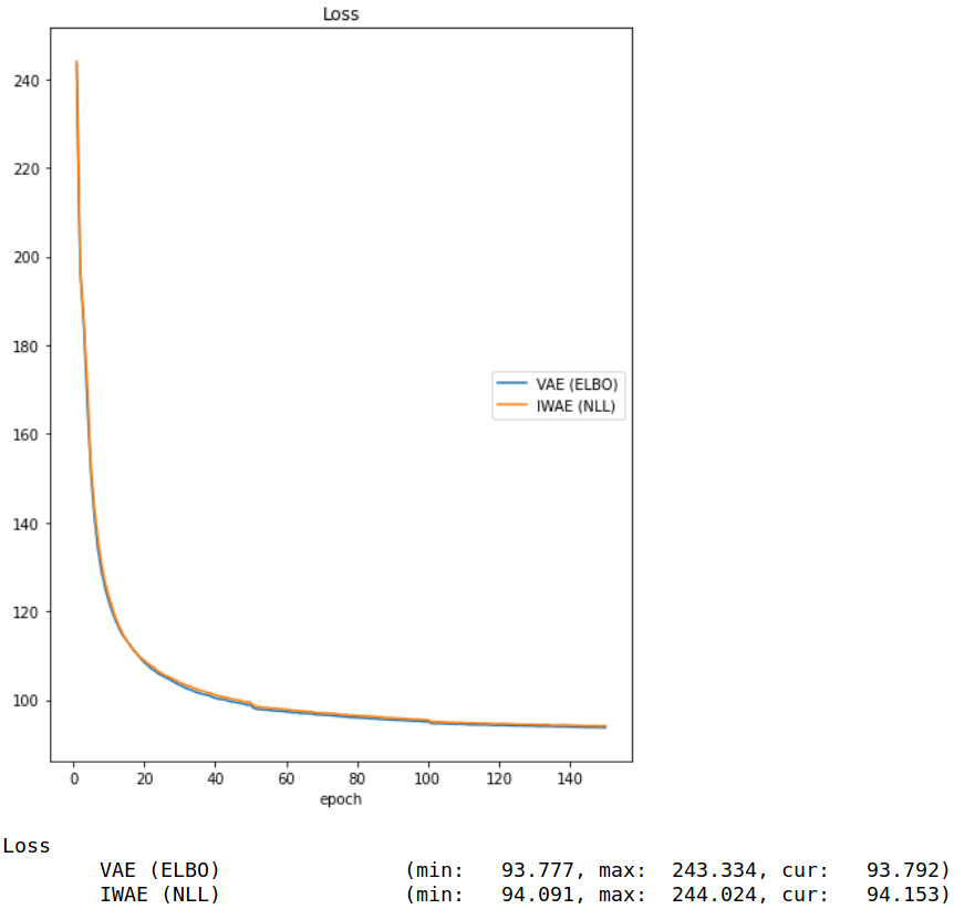
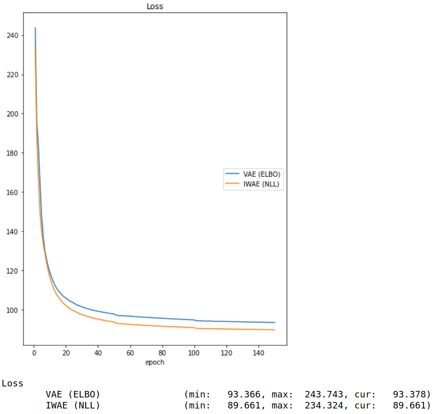
\(\textbf{k=1}\) Training k=1 \(\textbf{k=10}\) Training k=10

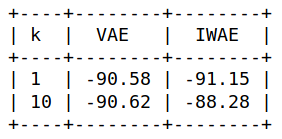
Note that during training, we compared the loss of the VAE (ELBO) with the loss of the IWAE (empirical estimate of marginal log-likelihood). Clearly, for \(k=1\) these losses are nearly equal (as expected). For \(k=10\), the difference is much greater (also expected). Now let’s compare the marginal log-likelihood on the test samples. Since the marginal log-likelihood estimator gets more accurate with increasing \(k\), we set \(k=200\) for the evaluation on the test set:

Code
from prettytable import PrettyTable


def compute_test_log_likelihood(test_dataset, trained_vae, trained_iwae, k=200):
    device = 'cuda' if torch.cuda.is_available() else 'cpu'

    data_loader = DataLoader(test_dataset, batch_size=20,
                             shuffle=True, num_workers=12)
    trained_vae.to(device)
    trained_iwae.to(device)

    avg_marginal_ll_VAE = 0
    avg_marginal_ll_IWAE = 0
    for x in data_loader:
        marginal_ll, _ = trained_vae.compute_marginal_log_likelihood(x.to(device), k)
        avg_marginal_ll_VAE += marginal_ll.item() / len(data_loader)

        marginal_ll, _ = trained_iwae.compute_marginal_log_likelihood(x.to(device), k)
        avg_marginal_ll_IWAE += marginal_ll.item() / len(data_loader)
    return avg_marginal_ll_VAE, avg_marginal_ll_IWAE


out_table = PrettyTable(["k", "VAE", "IWAE"])
test_ds = Binarized_MNIST('./data', train=False, download=True,
                                  transform=transforms.ToTensor())
for k in list_of_ks:
    # load models
    trained_vae = torch.load(f'./results/trained_vae_{k}.pth')
    trained_iwae = torch.load(f'./results/trained_iwae_{k}.pth')
    # compute average marginal log-likelihood on test dataset
    ll_VAE, ll_IWAE = compute_test_log_likelihood(test_ds, trained_vae, trained_iwae)
    out_table.add_row([k, np.round(ll_VAE, 2), np.round(ll_IWAE, 2)])
print(out_table)

Results NLL

Similar to the paper, the IWAE benefits from an increased \(k\) whereas the VAE performs nearly equal.

Visualizations

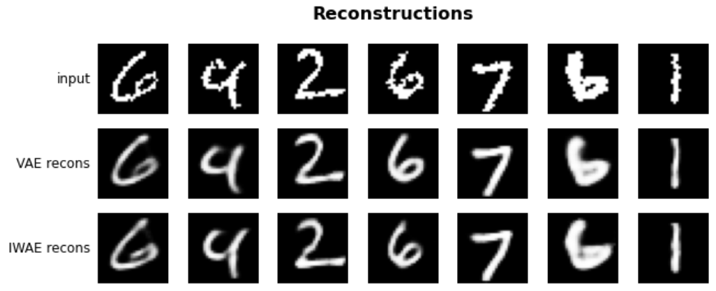
Lastly, let’s make some nice plots. Note that the differences are very subtle and it’s not very helpful to make an argument based on the following visualization. They mainly serve as a verification that both models do something useful.

  • Reconstructions
Code
import matplotlib.pyplot as plt
from matplotlib.gridspec import GridSpec


def plot_reconstructions(vae_model, iwae_model, dataset, SEED=1):
    np.random.seed(SEED)
    device = 'cuda' if torch.cuda.is_available() else 'cpu'

    vae_model.to(device)
    iwae_model.to(device)

    n_samples = 7
    i_samples = np.random.choice(range(len(dataset)), n_samples, replace=False)

    fig = plt.figure(figsize=(10, 4))
    plt.suptitle("Reconstructions", fontsize=16, y=1, fontweight='bold')
    for counter, i_sample in enumerate(i_samples):
        orig_img = dataset[i_sample]
        # plot original img
        ax = plt.subplot(3, n_samples, 1 + counter)
        plt.imshow(orig_img[0], vmin=0, vmax=1, cmap='gray')
        plt.axis('off')
        if counter == 0:
            ax.annotate("input", xy=(-0.1, 0.5), xycoords="axes fraction",
                        va="center", ha="right", fontsize=12)
        # plot img reconstruction VAE
        [x_tilde, z, mu_z, log_var_z] = vae_model(orig_img.unsqueeze(0).to(device))
        ax = plt.subplot(3, n_samples, 1 + counter + n_samples)
        x_tilde = x_tilde.squeeze(0)[0].detach().cpu().numpy()
        plt.imshow(x_tilde[0], vmin=0, vmax=1, cmap='gray')
        plt.axis('off')
        if counter == 0:
            ax.annotate("VAE recons", xy=(-0.1, 0.5), xycoords="axes fraction",
                        va="center", ha="right", fontsize=12)
        # plot img reconstruction IWAE
        [x_tilde, z, mu_z, log_var_z] = iwae_model(orig_img.unsqueeze(0).to(device))
        ax = plt.subplot(3, n_samples, 1 + counter + 2*n_samples)
        x_tilde = x_tilde.squeeze(0)[0].detach().cpu().numpy()
        plt.imshow(x_tilde[0], vmin=0, vmax=1, cmap='gray')
        plt.axis('off')
        if counter == 0:
            ax.annotate("IWAE recons", xy=(-0.1, 0.5), xycoords="axes fraction",
                        va="center", ha="right", fontsize=12)
    return


k = 10
trained_vae = torch.load(f'./results/trained_vae_{k}.pth')
trained_iwae = torch.load(f'./results/trained_iwae_{k}.pth')
plot_reconstructions(trained_vae, trained_iwae , test_ds)

Reconstructions k=10
  • Latent Traversals
Code
def plot_latent_traversal(vae_model, iwae_model, dataset, SEED=1):
    np.random.seed(SEED)
    device = 'cuda' if torch.cuda.is_available() else 'cpu'

    vae_model.to(device)
    iwae_model.to(device)

    n_samples = 128
    i_samples = np.random.choice(range(len(dataset)), n_samples, replace=False)
    img_batch = torch.cat([dataset[i].unsqueeze(0) for i in i_samples], 0)
    img_batch = img_batch.to(device)
    # generate latent traversals
    n_pert, pert_min_max, n_lats = 5, 2, 5
    img_trav_vae = vae_model.create_latent_traversal(img_batch, n_pert, pert_min_max, n_lats)
    img_trav_iwae = iwae_model.create_latent_traversal(img_batch, n_pert, pert_min_max, n_lats)

    fig = plt.figure(figsize=(12, 7))
    n_rows, n_cols = n_lats + 1, 2*n_pert + 1
    gs = GridSpec(n_rows, n_cols + 1)
    plt.suptitle("Latent Traversals", fontsize=16, y=1, fontweight='bold')
    for row_index in range(n_lats):
        for col_index in range(n_pert):
            img_rec_VAE = img_trav_vae[row_index][col_index]
            img_rec_IWAE = img_trav_iwae[row_index][col_index]

            ax = plt.subplot(gs[row_index, col_index])
            plt.imshow(img_rec_VAE[0].detach(), cmap='gray', vmin=0, vmax=1)
            plt.axis('off')

            if row_index == 0 and col_index == int(n_pert//2):
                plt.title('VAE', fontsize=14, y=1.1)

            ax = plt.subplot(gs[row_index, col_index + n_pert + 1])
            plt.imshow(img_rec_IWAE[0].detach(), cmap='gray', vmin=0, vmax=1)
            plt.axis('off')
            if row_index == 0 and col_index == int(n_pert//2):
                plt.title('IWAE', fontsize=14, y=1.1)
    # add pertubation magnitude
    for ax in [plt.subplot(gs[n_lats, 0:5]), plt.subplot(gs[n_lats, 6:11])]:
        ax.annotate("pertubation magnitude", xy=(0.5, 0.6), xycoords="axes fraction",
                    va="center", ha="center", fontsize=10)
        ax.set_frame_on(False)
        ax.axes.set_xlim([-1.15 * pert_min_max, 1.15 * pert_min_max])
        ax.xaxis.set_ticks([-pert_min_max, 0, pert_min_max])
        ax.xaxis.set_ticks_position("top")
        ax.xaxis.set_tick_params(direction="inout", pad=-16)
        ax.get_yaxis().set_ticks([])
    # add latent coordinate traversed annotation
    ax = plt.subplot(gs[0:n_rows-1, n_cols])
    ax.annotate("latent coordinate traversed", xy=(0.4, 0.5), xycoords="axes fraction",
                    va="center", ha="center", fontsize=10, rotation=90)
    plt.axis('off')
    return


k = 10
trained_vae = torch.load(f'./results/trained_vae_{k}.pth')
trained_iwae = torch.load(f'./results/trained_iwae_{k}.pth')
plot_latent_traversal(trained_vae, trained_iwae , test_ds)

Latent Traversal k=10

Footnotes

  1. Since the variance \(\text{diag} \left(\boldsymbol{\sigma}^2_{\text{E}}\right)\) needs to be greater than 0, we typically set the output to the variance in logarithmic units.↩︎