Model Description
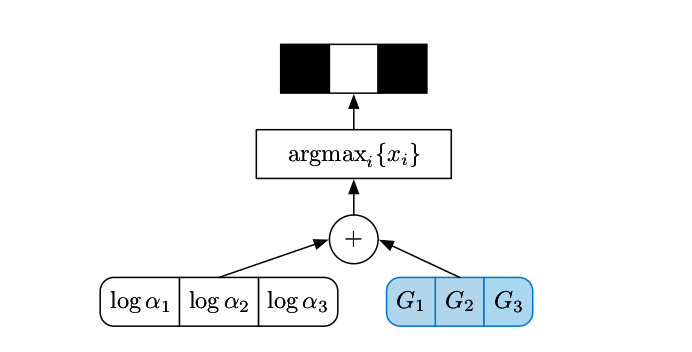
The Concrete distribution builds upon the (very old) Gumbel-Max trick that allows for a reparametrization of a categorical distribution into a deterministic function over the distribution parameters and an auxiliary noise distribution. The problem within this reparameterization is that it relies on an \(\text{argmax}\)-operation such that backpropagation remains out of reach. Therefore, Maddison et al. (2016) propose to use the \(\text{softmax}\)-operation as a continuous relaxation of the \(\text{argmax}\). This idea has been concurrently developed at the same time by Jang et al. (2016) who called it the Gumbel-Softmax trick.
Gumbel-Max Trick
The Gumbel-Max trick basically refactors sampling of a deterministic random variable into a component-wise addition of the discrete distribution parameters and an auxiliary noise followed by \(\text{argmax}\), i.e.,
\[
\begin{align}
\text{Sampling }&z \sim \text{Cat} \left(\alpha_1, \dots, \alpha_N \right)
\text{ can equally expressed as } z = \arg\max_{k} \Big(\log\alpha_k + G_k\Big)\\
&\text{with } G_k \sim \text{Gumbel Distribution}\left(\mu=0, \beta=1 \right)
\end{align}
\]
Derivation: Let’s take a closer look on how and why that works. Firstly, we show that samples from \(\text{Cat} \left(\alpha_1, \dots, \alpha_N \right)\) are equally distributed to
\[
z = \arg \min_{k} \frac {\epsilon_k}{\alpha_k} \quad \text{with} \quad
\epsilon_k \sim \text{Exp}\left( 1 \right)
\]
Therefore, we observe that each term inside the \(\text{argmin}\) is independent exponentially distributed with (easy proof)
\[
\frac {\epsilon_k}{\alpha_k} \sim \text{Exp} \Big( \alpha_k \Big)
\]
The next step is to show that the index of the variable which achieves the minimum is distributed according to the categorical distribution (easy proof)
\[
\arg \min_{k} \frac {\epsilon_k}{\alpha_k} = P \left( k | z_k = \min \{ z_1, \dots, z_N \} \right) = \frac
{\alpha_k}{\sum_{i=1}^N \alpha_i}
\]
A nice feature of this formulation is that the categorical distribution parameters \(\{\alpha_i\}_{i=1}^N\) do not need to be normalized before reparameterization as normalization is ensured by the factorization itself. Lastly, we simply reformulate this mapping by applying the log and multiplying by minus 1
\[
z = \arg \min_{k} \frac {\epsilon_k}{\alpha_k} =\arg \min_k \Big(\log \epsilon_k -
\log \alpha_k \Big) = \arg \max_k \Big(\log \alpha_k - \log \epsilon_k\Big)
\]
This looks already very close to the Gumbel-Max trick defined above. Remind that to generate exponential distributed random variables, we can simply transform uniformly distributed samples of the unit interval as follows
\[
\epsilon_k = -\log u_k \quad \text{with} \quad u_k \sim
\text{Uniform Distribution} \Big(0, 1\Big)
\]
Thus, we get that
\[
- \log \epsilon_k = - \log \Big( - \log u_k \Big) = G_k \sim
\text{Gumbel Distribution} \Big( \mu=0, \beta=1 \Big)
\]
Gumbel-Softmax Trick
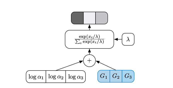
The problem in the Gumbel-Max trick is the \(\text{argmax}\)-operation as the derivative of \(\text{argmax}\) is 0 everywhere except at the boundary of state changes, where it is undefined. Thus, Maddison et al. (2016) use the temperature-valued \(\text{Softmax}\) as a continuous relaxation of the \(\text{argmax}\) computation such that
\[
\begin{align}
\text{Sampling }&z \sim \text{Cat} \left(\alpha_1, \dots, \alpha_N \right)
\text{ is relaxed cont. to } z_k = \frac {\exp \left( \frac {\log \alpha_k + G_k}{\lambda} \right)}
{\sum_{i=1}^N \exp \left( \frac {\log \alpha_i + G_i}{\lambda} \right)}\\
&\text{with } G_k \sim \text{Gumbel Distribution}\left(\mu=0, \beta=1 \right)
\end{align}
\]
where \(\lambda \in [0, \infty[\) is the temperature and \(\alpha_k \in [0,
\infty[\) are the categorical distribution parameters. The temperature can be understood as a hyperparameter that controls the sharpness of the \(\text{softmax}\), i.e., how much the winner-takes-all dynamics of the softmax is taken:
- \(\lambda \rightarrow 0\): \(\text{softmax}\) smoothly approaches discrete \(\text{argmax}\) computation
- \(\lambda \rightarrow \infty\): \(\text{softmax}\) leads to uniform distribution.
Note that the samples \(z_k\) obtained by this reparameterization follow a new family of distributions, the Concrete distribution. Thus, \(z_k\) are called Concrete random variables.
Intuition: To better understand the relationship between the Concrete distribution and the discrete categorical distribution, let’s look on an exemplary result. Remind that the \(\text{argmax}\) operation for a \(n\)-dimensional categorical distribution returns states on the vertices of the simplex
\[
\boldsymbol{\Delta}^{n-1} = \left\{ \textbf{x}\in \{0, 1\}^n \mid \sum_{k=1}^n x_k = 1 \right\}
\]
Concrete random variables are relaxed to return states in the interior of the simplex
\[
\widetilde{\boldsymbol{\Delta}}^{n-1} = \left\{ \textbf{x}\in [0, 1]^n \mid \sum_{k=1}^n x_k = 1 \right\}
\]
The image below shows how the distribution of concrete random variables changes for an exemplary discrete categorical distribution \((\alpha_1, \alpha_2,
\alpha_3) = (2, 0.5, 1)\) and different temperatures \(\lambda\).
Relationship between Concrete and Discrete Variables: A discrete distribution with unnormalized probabilities \((\alpha_1, \alpha_2, \alpha_3) = (2, 0.5, 1)\) and three corresponding Concrete densities at increasing temperatures \(\lambda\).
Taken from Maddison et al. (2016). |
Concrete Distribution
While the Gumbel-Softmax trick defines how to obtain samples from a Concrete distribution, Maddison et al. (2016) provide a definition of its density and prove some nice properties:
Definition: The Concrete distribution \(\text{X} \sim
\text{Concrete}(\boldsymbol{\alpha}, \lambda)\) with temperature \(\lambda \in
[0, \infty[\) and location \(\boldsymbol{\alpha} =
\begin{bmatrix} \alpha_1 & \dots & \alpha_n \end{bmatrix} \in [0, \infty]^{n}\) has a density
\[
p_{\boldsymbol{\alpha}, \lambda} (\textbf{x}) = (n-1)! \lambda^{n-1} \prod_{k=1}^n
\left( \frac {\alpha_k x_k^{-\lambda - 1}} {\sum_{i=1}^n \alpha_i x_i^{-\lambda}} \right)
\]
Nice Properties and their Implications:
Reparametrization: Instead of sampling directly from the Concrete distribution, one can obtain samples by the following deterministic (\(d\)) reparametrization
\[
X_k \stackrel{d}{=} \frac {\exp \left( \frac {\log \alpha_k + G_k}{\lambda} \right)}
{\sum_{i=1}^N \exp \left( \frac {\log \alpha_i + G_i}{\lambda} \right)} \quad
\text{with} \quad G_k \sim \text{Gumbel}(0, 1)
\]
This property ensures that we can easily compute unbiased low-variance gradients w.r.t. the location parameters \(\boldsymbol{\alpha}\) of the Concrete distribution.
Rounding: Rounding a Concrete random variable results in the discrete random variable whose distribution is described by the logits \(\log \alpha_k\)
\[
P (\text{X}_k > \text{X}_i \text{ for } i\neq k) = \frac {\alpha_k}{\sum_{i=1}^n \alpha_i}
\]
This property again indicates the close relationship between concrete and discrete distributions.
Convex eventually:
\[
\text{If } \lambda \le \frac {1}{n-1}, \text{ then } p_{\boldsymbol{\alpha},
\lambda} \text{ is log-convex in } x
\]
This property basically tells us if \(\lambda\) is small enough, there are no modes in the interior of the probability simplex.
Discrete-Latent VAE
One use-case of the Concrete distribution and its reparameterization is the training of an variational autoencoder (VAE) with a discrete latent space. The main idea is to use the Concrete distribution during training and use discrete sampled latent variables at test-time. An obvious limitation of this approach is that during training non-discrete samples are returned such that our model needs to be able to handle continuous variables. Let’s dive into the discrete-latent VAE described by Maddison et al. (2016).
We assume that we have a dataset \(\textbf{X} =
\{\textbf{x}^{(i)}\}_{i=1}^N\) of \(N\) i.i.d. samples \(\textbf{x}^{(i)}\) which were generated by the following process:
- We sample a one-hot latent vector \(\textbf{d}\in\{0, 1\}^{K}\) from a categorical prior distribution \(P_{\boldsymbol{a}} (\textbf{d})\).
- We use our sample \(\textbf{d}^{(i)}\) and put it into the scene model \(p_{\boldsymbol{\theta}}(\textbf{x}|\textbf{d})\) from which we sample to generate the observed image \(\textbf{x}^{(i)}\).
As a result, the marginal likelihood of an image can be stated as follows
\[
p_{\boldsymbol{\theta}, \boldsymbol{a}} (\textbf{x}) = \mathbb{E}_{\textbf{d}
\sim P_{\boldsymbol{a}}(\textbf{d})} \Big[ p_{\boldsymbol{\theta}} (\textbf{x} |
\textbf{d}) \Big] = \sum P_{\boldsymbol{a}} \left(\textbf{d}^{(i)} \right) p_{\boldsymbol{\theta}} \left( \textbf{x} |
\textbf{d}^{(i)} \right),
\]
where the sum is over all possible \(K\) dimensional one-hot vectors. In order to recover this generative process, we introduce a variational approximation \(Q_{\boldsymbol{\phi}} (\textbf{d}|\textbf{x})\) of the true, but unknown posterior. Now we exchange the sampling distribution towards this approximation
\[
p_{\boldsymbol{\theta}, \boldsymbol{a}} (\textbf{x}) = \sum
\frac {p_{\boldsymbol{\theta}, \boldsymbol{a}} \left(\textbf{x}, \textbf{d}^{(i)}
\right)}{Q_{\boldsymbol{\phi}} \left(\textbf{d}^{(i)} | \textbf{x}\right)}
Q_{\boldsymbol{\phi}} \left(\textbf{d}^{(i)} | \textbf{x}\right) =
\mathbb{E}_{\textbf{d} \sim Q_{\boldsymbol{\phi}} \left(\textbf{d} |
\textbf{x}\right)} \left[ \frac {p_{\boldsymbol{\theta}, \boldsymbol{a}} \left(\textbf{x}, \textbf{d}
\right)}{Q_{\boldsymbol{\phi}} \left(\textbf{d} | \textbf{x}\right)} \right]
\]
Lastly, applying Jensen’s inequality on the log-likelihood leads to the evidence lower bound (ELBO) objective of VAEs
\[
\log p_{\boldsymbol{\theta}, \boldsymbol{a}} (\textbf{x}) =
\log \left(
\mathbb{E}_{\textbf{d} \sim Q_{\boldsymbol{\phi}} \left(\textbf{d} |
\textbf{x}\right)} \left[ \frac {p_{\boldsymbol{\theta}, \boldsymbol{a}} \left(\textbf{x}, \textbf{d}
\right)}{Q_{\boldsymbol{\phi}} \left(\textbf{d} | \textbf{x}\right)} \right]\right)
\ge
\mathbb{E}_{\textbf{d} \sim Q_{\boldsymbol{\phi}} \left(\textbf{d} |
\textbf{x}\right)} \left[ \log \frac {p_{\boldsymbol{\theta}, \boldsymbol{a}} \left(\textbf{x}, \textbf{d}
\right)}{Q_{\boldsymbol{\phi}} \left(\textbf{d} | \textbf{x}\right)} \right]
= \mathcal{L}^{\text{ELBO}}
\]
While we are able to compute this objective, we cannot simply optimize it using standard automatic differentiation (AD) due to the discrete sampling operations. The concrete distribution comes to rescue: Maddison et al. (2016) propose to relax the terms \(P_{\boldsymbol{a}}(\textbf{d})\) and \(Q_{\boldsymbol{\phi}}(\textbf{d}|\textbf{x})\) using concrete distributions instead, leading to the relaxed objective
\[
\mathcal{L}^{\text{ELBO}}=
\mathbb{E}_{\textbf{d} \sim Q_{\boldsymbol{\phi}} \left(\textbf{d} |
\textbf{x}\right)} \left[ \log \frac {p_{\boldsymbol{\theta}} \left(\textbf{x}| \textbf{d}
\right) P_{\boldsymbol{a}} (\textbf{d}) }{Q_{\boldsymbol{\phi}} \left(\textbf{d} | \textbf{x}\right)} \right]
\stackrel{\text{relax}}{\rightarrow}
\mathbb{E}_{\textbf{z} \sim q_{\boldsymbol{\phi}, \lambda_1} \left(\textbf{z} |
\textbf{x}\right)} \left[ \log \frac {p_{\boldsymbol{\theta}} \left(\textbf{x}| \textbf{z}
\right) p_{\boldsymbol{a}, \lambda_2} (\textbf{z}) }{q_{\boldsymbol{\phi}, \lambda_1} \left(\textbf{z} | \textbf{x}\right)} \right]
\]
Then, during training we optimize the relaxed objective while during test time we evaluate the original objective including discrete sampling operations. The really neat thing here is that switching between the two modes works out of the box: we only need to switch between the \(\text{softmax}\) and \(\text{argmax}\) operations.
| Discrete-Latent VAE Architecture |
Things to beware of: Maddison et al. (2016) noted that naively implementing [the relaxed objective] will result in numerical issues. Therefore, they give some implementation hints in Appendix C:
Log-Probabilties of Concrete Variables can suffer from underflow: Let’s investigate why this might happen. The log-likelihood of a concrete variable \(\textbf{z}\) is given by
\[
\begin{align}
\log p_{\boldsymbol{\alpha}, \lambda} (\textbf{z}) =& \log \Big((K-1)! \Big) + (K-1) \log \lambda
+ \left(\sum_{i=1}^K \log \alpha_i + (-\lambda - 1) \log z_i \right) \\
&- K \log \left(\sum_{i=1}^K \exp\left( \log \alpha_i - \lambda \log z_i\right)\right)
\end{align}
\]
Now let’s remind that concrete variables are pushing towards one-hot vectors (when \(\lambda\) is set accordingly), i.e., due to rounding/underflow we might get some \(z_i=0\). This is problematic, since the \(\log\) is not defined in this case.
To circumvent this, Maddison et al. (2016) propose to work with Concrete random variables in log-space, i.e., to use the following reparameterization
\[
y_i = \frac {\log \alpha_i + G_i}{\lambda} - \log \left( \sum_{i=1}^K \exp
\left( \frac {\log \alpha_i + G_i}{\lambda} \right) \right)
\quad G_i \sim \text{Gumbel}(0, 1)
\]
The resulting random variable \(\textbf{y}\in\mathbb{R}^K\) has the property that \(\exp(Y) \sim \text{Concrete}\left(\boldsymbol{\alpha}, \lambda \right)\), therefore they denote \(Y\) as an \(\text{ExpConcrete}\left(\boldsymbol{\alpha},
\lambda\right)\). Accordingly, the log-likelihood \(\log
\kappa_{\boldsymbol{\alpha}, \lambda}\) of a variable ExpConcrete variable \(\textbf{y}\) is given by
\[
\begin{align}
\log p_{\boldsymbol{\alpha}, \lambda} (\textbf{y}) =& \log \Big((K-1)! \Big) + (K-1) \log \lambda
+ \left(\sum_{i=1}^K \log \alpha_i + (\lambda - 1) y_i \right) \\
&- n \log \left(\sum_{i=1}^n \exp\left( \log \alpha_i - \lambda y_i\right)\right)
\end{align}
\]
This reparameterization does not change our approach due to the fact that the KL terms of a variational loss are invariant under invertible transformations, i.e., since \(\exp\) is invertible, the KL divergence between two \(\text{ExpConcrete}\) is the same the KL divergence between two \(\text{Concrete}\) distributions.
Working with \(\text{ExpConcrete}\) random variables: Remind the relaxed objective
\[
\mathcal{L}^{\text{ELBO}}_{rel} =
\mathbb{E}_{\textbf{z} \sim q_{\boldsymbol{\phi}, \lambda_1} \left(\textbf{z} |
\textbf{x}\right)} \left[
\log p_{\boldsymbol{\theta}} \left( \textbf{x} | \textbf{z}\right) + \log
\frac{
p_{\boldsymbol{a}, \lambda_2} (\textbf{z})
} {q_{\boldsymbol{\phi},
\lambda_1} \left(\textbf{z} | \textbf{x}\right)}
\right]
\]
Now let’s exchange the \(\text{Concrete}\) by \(\text{ExpConcrete}\) distributions
\[
\mathcal{L}^{\text{ELBO}}_{rel} =
\mathbb{E}_{\textbf{y} \sim \kappa_{\boldsymbol{\phi}, \lambda_1} \left(\textbf{z} |
\textbf{x}\right)} \left[
\log p_{\boldsymbol{\theta}} \left( \textbf{x} | \exp(\textbf{y})\right) + \log
\frac{
\rho_{\boldsymbol{a}, \lambda_2} (\textbf{y})
} {\kappa_{\boldsymbol{\phi},
\lambda_1} \left(\textbf{z} | \textbf{y}\right)}
\right],
\]
where \(\rho_{\boldsymbol{a}, \lambda_2} (\textbf{y})\) is the density of an \(\text{ExpConcrete}\) corresponding to the \(\text{Concrete}\) distribution \(p_{\boldsymbol{a}, \lambda_2} (\textbf{z})\). Thus, during the implementation we will simply use \(\text{ExpConcrete}\) random variables \(\textbf{y}\) as random variables and then perform an \(\exp\) computation before putting them through the decoder.
Choosing the temperature \(\lambda\): Maddison et al. (2016) note that the success of the training heavily depends on the choice of temperature. It is rather intuitive that the relaxed nodes should not be able to represent precise real valued mode in the interior of the probability simplex, since otherwise the model is designed to fail. In other words, the only modes of the concrete distributions should be at the vertices of the probability simplex. Fortunately, Maddison et al. (2016) proved that
\[
\text{If } \lambda \le \frac {1}{n-1}, \text{ then } p_{\boldsymbol{\alpha},
\lambda} \text{ is log-convex in } x
\]
In other words, if we keep \(\lambda \le \frac {1}{n-1}\), there are no modes in the interior. However, Maddison et al. (2016) note that in practice, this upper-bound on \(\lambda\) might be too tight, e.g., they found for \(n=4\) that \(\lambda=1\) was the best temperature and in \(n=8\), \(\lambda=\frac {2}{3}\). As a result, they recommend to rather explore \(\lambda\) as tuneable hyperparameters.
Last note about the temperature \(\lambda\): They found that choosing different temperatures \(\lambda_1\) and \(\lambda_2\) for the posterior \(\kappa_{\boldsymbol{\alpha}, \lambda_1}\) and prior \(\rho_{\boldsymbol{a},
\lambda_2}\) could dramatically improve the results.
