Why should a MSE loss be avoided after a sigmoid layer?

MSE loss after a sigmoid layer leads to the vanishing gradients problem in cases where the outputs of the sigmoid layer are close to \(0\) or \(1\) irrespective of the true probability/label. I.e., in the extreme case where the network output is something close to zero while the true label is 1, gradients w.r.t. network parameters are close to zero.

Derivation

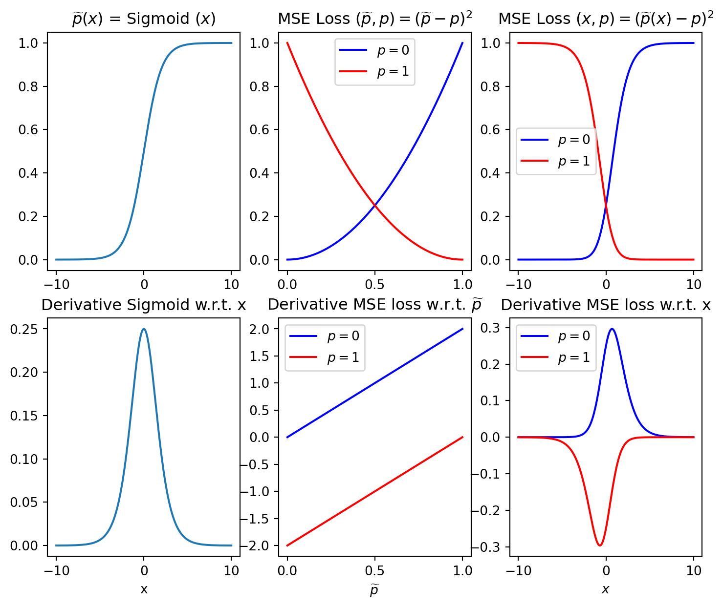
Let’s denote the output of the network by \(\widetilde{\textbf{p}} \in [0, 1]^{N}\) (for estimated probabilities) and the input to the sigmoid \(\textbf{x}\in \mathbb{R}^{N}\) (i.e., layer output before sigmoid is applied)

\[ \textbf{p} = \text{Sigmoid} (\textbf{x}) = \frac {1}{1 + \exp \left({-\textbf{x}}\right)} \]

Now suppose that \(\textbf{p}\in [0, 1]^{N}\) denotes the true probabilities, then applying the MSE loss gives

\[ \text{MSE loss} \left(\widetilde{\textbf{p}}, \textbf{p}\right) =J\left(\widetilde{\textbf{p}}, \textbf{p}\right) = \sum_{i=1}^N \left(\widetilde{p}_i - p_i \right)^2, \]

The gradient w.r.t. network parameters will be proportional to the gradient w.r.t. \(\textbf{x}\) (backpropagation rule) which is as follows

\[ \frac {\partial J \left(\widetilde{\textbf{p}}, \textbf{p}\right)}{\partial x_i} = \sum_{j=1}^N \frac {\partial J}{\partial p_j} \cdot \frac {\partial p_j}{\partial x_j} = 2 \left(\widetilde{p}_i - p_i \right) \cdot \frac {\partial p_i}{\partial x_i} = 2 \left(\widetilde{p}_i - p_i \right) \cdot p_i (1 - p_i) \]

Here we can directly see that even if the absolute error approaches 1, i.e., \(\left(\widetilde{p}_i - p_i \right)\rightarrow 1\), the gradient vanishes for \(p_i\rightarrow 1\) and \(p_i\rightarrow 0\).

Let’s derive the gradient of the sigmoid using substitution and the chain rule

\[ \begin{align} \frac {\partial p_i} {\partial x_i} &= \frac {\partial u}{\partial t} \cdot \frac {\partial t}{\partial x} \quad \text{with} \quad u(t) = t^{-1}, \quad t(x_i) = 1 + \exp{(-x_i)}\\ &= -t^{-2} \cdot \left(-\exp{x_i}\right) = \frac {exp\left(-x_i\right)}{\left(1 + \exp\left(-x_i\right)\right)^2}\\ &= \underbrace{\frac {1}{1 + \exp \left( -x \right)}}_{p_i} \underbrace{\frac {\exp (-x_i)}{1+exp(-x_i)}}_{1-p_i} = p_i \left(1 - p_i \right) \end{align} \]

Visualization

Let’s write a nice visualization using pytorch’s autograd.

import torch
from torch import nn
import matplotlib.pyplot as plt


def make_visualization():
    p0, p1 = 0, 1  # true probability

    points = torch.arange(-10, 10, step=0.01)
    # create variables to track gradients
    grad_points = nn.Parameter(points, requires_grad=True)
    p_tilde_0 = nn.Parameter(torch.sigmoid(points), requires_grad=True)
    p_tilde_1 = nn.Parameter(torch.sigmoid(points), requires_grad=True)
    grad_points_p0_x = nn.Parameter(points, requires_grad=True)
    grad_points_p1_x = nn.Parameter(points, requires_grad=True)

    # computations over which gradients are calculated
    out_sigmoid = torch.sigmoid(grad_points)
    MSE_loss_p0_p = (p_tilde_0 - p0)**2
    MSE_loss_p1_p = (p_tilde_1 - p1)**2
    MSE_loss_p0_x = (torch.sigmoid(grad_points_p0_x) - p0)**2
    MSE_loss_p1_x = (torch.sigmoid(grad_points_p1_x) - p1)**2
    # calculate gradients
    out_sigmoid.sum().backward()
    MSE_loss_p0_p.sum().backward()
    MSE_loss_p1_p.sum().backward()
    MSE_loss_p0_x.sum().backward()
    MSE_loss_p1_x.sum().backward()

    fig = plt.figure(figsize=(9,8))
    # sigmoid
    plt.subplot(3, 3, 1)
    plt.plot(grad_points.detach().numpy(), out_sigmoid.detach().numpy())
    plt.title(r'$\widetilde{p}(x)$ = Sigmoid $(x)$')
    # MSE loss w.r.t. \widetilde{p}
    plt.subplot(3, 3, 2)
    plt.plot(p_tilde_0.detach().numpy(), MSE_loss_p0_p.detach().numpy(),
             color='blue', label=r'$p=$' + f'{p0}')
    plt.plot(p_tilde_1.detach().numpy(), MSE_loss_p1_p.detach().numpy(),
             color='red', label=r'$p=$' + f'{p1}')
    plt.legend()
    plt.title(r'MSE Loss $(\widetilde{p}, p) = (\widetilde{p} - p)^2$')
    plt.subplots_adjust(bottom=-0.2)
    # MSE loss w.r.t. x
    plt.subplot(3, 3, 3)
    plt.plot(grad_points_p0_x.detach().numpy(), MSE_loss_p0_x.detach().numpy(),
             color='blue', label=r'$p=$' + f'{p0}')
    plt.plot(grad_points_p1_x.detach().numpy(), MSE_loss_p1_x.detach().numpy(),
             color='red', label=r'$p=$' + f'{p1}')
    plt.legend()
    plt.title(r'MSE Loss $(x, p) = (\widetilde{p}(x) - p)^2$')
    # derivative of sigmoid
    plt.subplot(3, 3, 4)
    plt.plot(grad_points.detach().numpy(), grad_points.grad)
    plt.title(r'Derivative Sigmoid w.r.t. x')
    plt.xlabel('x')
    # derivative of MSE loss w.r.t. \widetilde{p}
    plt.subplot(3, 3, 5)
    plt.plot(p_tilde_0.detach().numpy(), p_tilde_0.grad, color='blue',
             label=r'$p=$' + f'{p0}')
    plt.plot(p_tilde_1.detach().numpy(), p_tilde_1.grad, color='red',
             label=r'$p=$' + f'{p1}')
    plt.xlabel(r'$\widetilde{p}$')
    plt.title(r'Derivative MSE loss w.r.t. $\widetilde{p}$')
    plt.legend()
    # derivative of MSE Loss w.r.t x
    plt.subplot(3, 3, 6)
    plt.plot(grad_points_p0_x.detach().numpy(), grad_points_p0_x.grad,
             color='blue', label=r'$p=$' + f'{p0}')
    plt.plot(grad_points_p1_x.detach().numpy(), grad_points_p1_x.grad,
             color='red', label=r'$p=$' + f'{p1}')
    plt.xlabel(r'$x$')
    plt.title(r'Derivative MSE loss w.r.t. x')
    plt.legend()
    return

make_visualization()